Building Micrograd A Walkthrough

Walkthrough of Karpathy’s Building Micrograd lesson

Conrad Gomes • April 15, 2026

I am working my way through Andrej Karpathy’s lecture: The spelled-out intro to neural networks and backpropagation: building micrograd. This post documents my setup, progress, and thoughts as I build a tiny autograd engine from scratch.

Environment Setup

To keep my system clean, I am using a standard Python virtual environment on macOS.

Create the environment: python3 -m venv .venv
Activate it: source .venv/bin/activate
Install dependencies: pip install jupyter numpy matplotlib graphviz torch
Launch Jupyter: jupyter notebook

Setup the first part of the python code with the following:

import math
import numpy as np
import matplotlib.pyplot as plt
%matplotlib inline
from graphviz import Digraph
import random

Troubleshooting

I ran into a couple of minor hiccups getting started:

Missing Modules inside Jupyter: I initially installed packages in one terminal but they weren’t showing up in the notebook.
- Fix: I opened a new terminal, sourced the venv, and ran pip install jupyter numpy matplotlib graphviz torch.
Matplotlib Font Cache: On the first run, Matplotlib paused to build its font cache.
- Observation: This is normal. If it persists for more than a minute, re-running the cell usually clears it.

Part 1: The Derivative

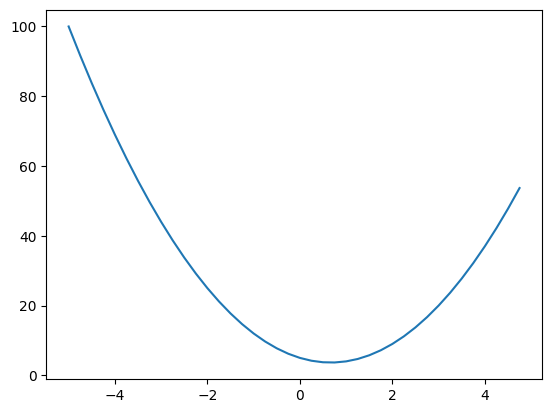
The first part is to gain an intuitive understanding of the derivative which is the fundamental mathematical operation for backpropagation. The goal is to understand the derivative intuitively by starting with a simple scalar function:

f(x) = 3x^2 - 4x + 5

We can implement this and tested it at $x = 3.0$ using a python function

def f(x):
    return 3*x**2 - 4*x + 5

Testing the function with 3.0 and 6.0 we can get the values of the quadratic function:

print(f(3.0))
print(f(6.0))

20.0
89.0

To gain an intuition of the function we use an array of values using numpy which we assign to xs. Then we get get the corresponding array of values that the function will return for each of those values by simply passing it to the function. Using matplotlib we take can plot the values of ys on the y-axis and xs on the x-axis

xs = np.arange(-5, 5, 0.25)

ys = f(xs)

plt.plot(xs, ys)
plt.savefig('multigrad-from-scratch-quadriatic-plt.png')

The derivative of a function is defined by the formula:

f'(x) = \lim_{h \to 0} \frac{f(x+h) - f(x)}{h}

Next, I calculated the numerical derivative at $x = 3.0$ by adding a tiny value $h$ and calculating the rise over run:

h = 0.00000000001
x = 3.0

def numerical_derivative_simple(f, x, h):
    # note that f, x, h are local variables
    # and not the same as global though they share the same names

    return (f(x+h) - f(x))/h

numerical_derivative_simple(f, x, h)

14.000178794049134

The symbolic derivative of $3x^2 - 4x + 5$ is $6x - 4$ . At $x = 3.0$ , this evaluates to $14$ . The numerical result is extremely close, which confirms the implementation is working.

To see how derivatives behave with multiple variables, we implement a more complex expression:

d = a \cdot b + c

# more complex

def d(a, b, c):
    # here a, b, and c are local variables in this function
    return a * b + c

# define a, b and c as values to be input to d
a = 2.0
b = -3.0
c = 10.0

# compute d0 with the values assigned above to check
d0 = d(a, b, c)
print(d0)

4.0

Now we can calculate the partial derivative of $d$ with respect to $a$ , first calculate $d$ for values $a$ , $b$ and $c$ . This will be called $d1$ . Next bump $a$ by very small $h$ keeping the other values of $b$ and $c$ the same and evaluate the expression as $d2$ . We implement this in the function numerical_partial_derivative_a. The lecture goes through this manually for each variable.

h = 0.0001

# define a, b and c as values to be input to d
a = 2.0
b = -3.0
c = 10.0

# Find derivative of d w.r.t a
def numerical_partial_derivative_a(d, a, b, c, h):
    d0 = d(a, b, c)
    # increment a with very small h
    d1 = d(a+h, b, c)
    
    return (d1 - d0)/h

# Calculate the partial derivative of a
numerical_partial_derivative_a(d, a, b, c, h)

-3.000000000010772

These results match the symbolic partial derivative of $d$ w.r.t $a$ . So the value we get is essentially the value of $b$ i.e. $-3.0$

\frac{\partial d}{\partial a}=b

# Find derivative of d w.r.t b
def numerical_partial_derivative_b(d, a, b, c, h):
    d0 = d(a, b, c)
    # increment b with very small h
    d1 = d(a, b+h, c)
    
    return (d1 - d0)/h

# Calculate the partial derivative of a
numerical_partial_derivative_b(d, a, b, c, h)

2.0000000000042206

These results match the symbolic partial derivative of $d$ w.r.t $b$ . So the value we get is essentially the value of $a$ i.e. $2.0$

\frac{\partial d}{\partial b}=a

# Find derivative of d w.r.t c
def numerical_partial_derivative_c(d, a, b, c, h):
    d0 = d(a, b, c)
    # increment b with very small h
    d1 = d(a, b, c+h)
    
    return (d1 - d0)/h

# Calculate the partial derivative of a
numerical_partial_derivative_c(d, a, b, c, h)

0.9999999999976694

These results match the symbolic partial derivative of $d$ w.r.t $c$ . So the value we get is essentially $1$

\frac{\partial d}{\partial c}=1

Part 2: The Framework

Here we build out a framework to model the mathematical operation. We will build out a Value class object to represent the values in the mathematical operation and model the operations as methods of this class. We also implement functions to help visualize the mathematical operation setting the stage for the next section of backpropagation.

class Value:
    def __init__(self, data, _children=(), _op='', label=''):
        self.data = data
        self.label = label
        self._prev = set(_children)
        self._op = _op
        self.grad = 0
        self._backward = lambda: None

    def __repr__(self):
        return f"Value(Data={self.data})"

    def __add__(self, other):
        other = other if isinstance(other, Value) else Value(other)
        out = Value(self.data + other.data, (self, other), '+')
        def _backward():
            self.grad += 1 * out.grad
            other.grad += 1 * out.grad
        out._backward = _backward
        return out

    def __sub__(self, other):
        return self + (-other)

    def __neg__(self):
        return self * -1;
        
    def __radd__(self,other):
        return self.__add__(other)

    def __mul__(self, other):
        other = other if isinstance(other, Value) else Value(other)
        out =  Value(self.data * other.data, (self, other), '*')
        def _backward():
            self.grad +=  other.data * out.grad
            other.grad += self.data * out.grad
        out._backward = _backward
        return out

    def __rmul__(self, other):
        return self * other

    def __truediv__(self, other):
        return self * other**-1

    def __pow__(self, other):
        assert isinstance(other, (int, float)), "only supporting int/float powers for now"
        out = Value(self.data**other, (self,), f'**{other}')

        def _backward():
            self.grad += (other * (self.data**(other-1))) * out.grad
        out._backward = _backward

        return out
    
    def exp(self):
        x = self.data
        out = Value(math.exp(x), (self,), 'exp')
        def _backward():
            self.grad += out.data * out.grad
        out._backward = _backward
        return out
        
    def tanh(self):
        t = (math.exp(2*self.data) - 1)/(math.exp(2*self.data) + 1)
        out =  Value(t, (self,), 'tanh')
        def _backward():
            self.grad += (1 - t**2) * out.grad;
        out._backward = _backward
        return out

    def backward(self):
        visited = set()
        topo = []
        def build_topo(v):
            if v not in visited:
                visited.add(v)
                for child in v._prev:
                    build_topo(child)
                topo.append(v)

        build_topo(self)

        self.grad = 1.0

        for node in reversed(topo):
            node._backward()

Store and Print Data

The lecture starts with defining a basic class which can be initialized with any floating point number. This is achieved by defining the constructor __init__ to take in a data argument to store the value. In order to be able to print object of this class we define a __repr__ method to print out the data owned by the class object. This gives us the ability to initialize a Value object and print it out as follows

a = Value(2.0)
print(a) # Output: Value(data=2.0)

Value(Data=2.0)

Python Concepts Learned:

__init__: This is the constructor. It sets up the initial data for each new Value object. (Python Docs: init)
__repr__: This method provides a readable string representation of the object. Without it, Python defaults to showing a memory address like <__main__.Value object at 0x...>. (Python Docs: repr)
f-strings (f"..."): I learned that the f prefix allows for “formatted strings,” where variables inside {} are evaluated and inserted directly into the text.

Implementing Mathematical Operators

Next we need to be able to perform the same operations we did with raw scalars, but using our Value objects within the framework. The class Value has methods __add__ and __mul__ to class to overload the + and * operators. For a full list of these special “dunder” (double underscore) methods, the Python Data Model documentation is the definitive resource.

With these dunder methods we should be able to acheive the addition and multiplication operations using the + and * operators:

a = Value(2.0)
b = Value(-3.0)
c = Value(10.0)

a + b # Output: Value(Data=-1.0)

Value(Data=-1.0)



ERROR! Session/line number was not unique in database. History logging moved to new session 3

a * b # Output: Value(Data=-6.0)

Value(Data=-6.0)

I also tested calling these “dunder” methods directly, which confirmed that a + b is just a more readable way of writing a.__add__(b):

a.__add__(b) # Output: Value(Data=-1.0)

Value(Data=-1.0)

Finally, I combined them into the same complex expression we used earlier:

d = a * b + c
print(d) # Output: Value(Data=4.0)

Value(Data=4.0)

Building Mathematical Expression Graph

The next step in the lecture is to represent mathematical expressions as graphs. By building this graph structure, we can track not just the result of a calculation, but exactly how it was constructed from its components.

The Value class object returned by a mathematical operation should store the Value objects that were used to obtain the returned object. The Value objects used to construct a new Value object can be considered as “children”.

The __init__ constructor of the Value class has a _children argument which signifies a tuple of Value objects which is used to create the Value object being constructed. This tuple is stored as a set in the self._prev = set(_children) initialization. Therefore in the __add__ and __mul__ methods we can see that the new resulting Value objects are initialized with a tuple consisting of self and other objects.

In the following example we construct a Value object e using a and b. We then print e._prev to see the “children” objects.

a = Value(2.0)
b = Value(-3.0)
e = a * b
print(e)
print(e._prev)

Value(Data=-6.0)
{Value(Data=2.0), Value(Data=-3.0)}

In addition to the constituent objects that create a Value object we also store the operator that lead to its construction. This is passed throught the _op argument. In the __add__ and __mul__ methods we pass in the + and * operator identifiers. We can also see the operator as follows:

print(e._op)

Visualizing The Mathematical Expression Graph

In order to visualize the mathematical expression graph the lecture proceeds to use graphviz we have already added the import statement i.e. from graphviz import Digraph above in the environment setup section.

Specifically:

graphviz: The Python library that acts as a wrapper for the Graphviz software.
Digraph: Short for Directed Graph. It is a class used to create graphs where the edges have arrows (direction), showing a relationship from one node to another (e.g., $A \to B$ ).

We define a function trace to return the nodes and edges of the graph

def trace(root):
    # builds a set of all nodes and edges in a graph
    nodes, edges = set(), set()

    def build(v):
        if v not in nodes:
            nodes.add(v)
            for child in v._prev:
                edges.add((child, v))
                build(child)
    
    build(root)
    return nodes, edges

def draw_dot(root):
    dot = Digraph(format='svg', graph_attr={'rankdir': 'LR'})

    nodes, edges = trace(root)
    for n in nodes:
        uid = str(id(n))
        # for any value in the graph, create a rectangular ('record') node for it
        dot.node(name = uid, label = "{%s | data % 4f | grad % 4f }" % (n.label, n.data, n.grad), shape = 'record')
        if n._op:
            # if this node is the result of some operation create an op node for it
            dot.node(name = uid + n._op, label = n._op)
            # and connect this node to it
            dot.edge(uid + n._op, uid)

    for n1, n2 in edges:
        # connect n1 to the op node of n2
        dot.edge(str(id(n1)), str(id(n2)) + n2._op)

    dot.render('graphexample', format='png')
    return dot

We extend the __init__ constructor to also take a label argument. This is used in the draw_dot function to name the Value objects which are depicted as rectangular nodes. Whenever a node is found to have a valid _op an operator node is created and connected to the record object. The children objects are connected to the operator node.

In order to test the visualization we create a complex mathematical expression. For objects holding the result object of an operation we have to explicitly assign the label e.g. for the object e which is created by multiplying objects a and b we have to set its label explicitly.

The expression below computes a Value object labelled L. We can use the draw_dot function to visualize it. The resulting visualization clearly shows the entire computational graph leading up to L:

Note: The visualization will also have a grad attribute which represents the gradient of the node which will be covered in the subsequent backpropogation sections.

a = Value(2.0, label='a')
b = Value(-3.0, label='b')
c = Value(10.0, label='c')
e = a * b; e.label='e'
d = e + c; d.label='d'
f = Value(-2.0, label='f')
L = d * f; L.label='L'

print(L)

Value(Data=-8.0)

draw_dot(L)

The `grad` part of the node will be computed after the manual backpropogation step

  Cell In[24], line 1
    The `grad` part of the node will be computed after the manual backpropogation step
        ^
SyntaxError: invalid syntax

Part 3: Manual Backpropogation

In this part we learn how to manually fill up the gradient for each of the Value objects in the graph. We use a staging function to demonstrate the gradient for each object. The staging function serves to verify the numerical computation of the gradient.

$dL/dL$

We start by calculating the gradient of the output $L$ with respect to itself. Using the definition of a derivative:

f'(x) = \lim_{h \to 0} \frac{f(x+h) - f(x)}{h}

If we consider $L$ as a function of itself, then:

\frac{dL}{dL} = \lim_{h \to 0} \frac{(L+h) - (L)}{h} = 1

Thus, we initialize L.grad = 1.0.

To confirm our manual calculations, we use a numerical approximation. By “bumping” a value by a tiny amount $h$ and observing the change in $L$ . Andrej refers to this as the lol() function in the lecture a staging area to verify our intuition numerically before we automate the process.

def lol():
    h = 0.001
    a = Value(2.0, label='a')
    b = Value(-3.0, label='b')
    c = Value(10.0, label='c')
    e = a * b; e.label='e'
    d = e + c; d.label='d'
    f = Value(-2.0, label='f')
    L = d * f; L.label='L'
    L1 = L.data

    a = Value(2.0, label='a');
    b = Value(-3.0, label='b');
    c = Value(10.0, label='c');
    e = a * b; e.label='e';
    d = e + c; d.label='d'
    f = Value(-2.0, label='f')
    L = d * f; L.label='L'
    L2 = L.data + h

    print((L2 - L1)/h)

lol()

1.000000000000334

We set L.grad to 1.0

L.grad = 1.0

$dL/dd$ and $dL/df$

Next, we calculate the gradients for the inputs of the final multiplication $L = d \cdot f$ . Here $L$ is a function of $d$ and $f$ .

Using the power rule for a product $f(x,y) = x \cdot y$ :

\frac{\partial f}{\partial x} = y, \quad \frac{\partial f}{\partial y} = x

Applying this to $L = d \cdot f$ :

\frac{dL}{dd} = f \quad \text{and} \quad \frac{dL}{df} = d

From our graph:

$f = -2.0$ , so d.grad = -2.0
$d = 4.0$ , so f.grad = 4.0

We can verify this with the lol() function by bumping d or f and checking the result. We show it for only d by bumping d.data by h below. The same can be verified for f.

When the operation at a node is a multiplication the gradient of the inputs is a multiplication of the output gradient with the other inputs. In the case of f the output gradient is 1.0 and the input 4.0 so the gradient f.grad is the multiplication of these two values. The same is applicable to d.

def lol():
    h = 0.001
    a = Value(2.0, label='a')
    b = Value(-3.0, label='b')
    c = Value(10.0, label='c')
    e = a * b; e.label='e'
    d = e + c; d.label='d'
    f = Value(-2.0, label='f')
    L = d * f; L.label='L'
    L1 = L.data

    a = Value(2.0, label='a');
    b = Value(-3.0, label='b');
    c = Value(10.0, label='c');
    e = a * b; e.label='e';
    d = e + c; d.label='d'; d.data += h
    f = Value(-2.0, label='f')
    L = d * f; L.label='L'
    L2 = L.data

    print((L2 - L1)/h)

lol()

-2.000000000000668

We set d.grad to -2.0 and f.grad to 4.0

d.grad = -2.0
f.grad = 4.0

$dL/de$ and $dL/dc$

Now we move deeper into the graph to calculate gradients for e and c. These nodes influence L through d, so we need to use the Chain Rule.

The Chain Rule states that if $f$ is a function of $y$ and $y$ is a function of $x$ then the derivative of $f$ w.r.t $x$ can be expressed as:

\frac{df}{dx} = \frac{df}{dy} \cdot \frac{dy}{dx}

For e, we want $\frac{dL}{de}$ . We know $\frac{dL}{dd}$ as computed in the above section. Therefore we only need to compute $\frac{dd}{de}$ to get $\frac{dL}{de}$ as per the chain rule:

\frac{dL}{de} = \frac{dL}{dd} \cdot \frac{dd}{de}

Since $d = e + c$ , the local derivative is:

\frac{dd}{de} = 1.0

So:

\frac{dL}{de} = -2.0 \cdot 1.0 = -2.0

Similarly for c:

\frac{dL}{dc} = \frac{dL}{dd} \cdot \frac{dd}{dc}

\frac{dd}{dc} = 1.0

\frac{dL}{dc} = -2.0 \cdot 1.0 = -2.0

Thus, e.grad = -2.0 and c.grad = -2.0. When the operation of the node is an addition the gradient of the inputs is the same as the value of gradient of the node.

e.grad = -2.0
c.grad = -2.0

$dL/da$ and $dL/db$

Finally, we backpropagate to a and b through e.

For a:

\frac{dL}{da} = \frac{dL}{de} \cdot \frac{de}{da}

Since $e = a \cdot b$ :

\frac{de}{da} = b

So:

\frac{dL}{da} = -2.0 \cdot -3.0 = 6.0

For b:

\frac{dL}{db} = \frac{dL}{de} \cdot \frac{de}{db}

\frac{de}{db} = a

So:

\frac{dL}{db} = -2.0 \cdot 2.0 = -4.0

Thus, a.grad = 6.0 and b.grad = -4.0.

a.grad = 6.0
b.grad = -4.0

draw_dot(L)

Single Step of Optimization Example

We can see the effect of a single step of optimization by trying to change the inputs to the expression by an amount in the direction of their gradients. The gradient gives us the ability to control the output L which is very useful to train neural networks. In the lecture we see that updating the values of a, b, c and f by a small amount 0.01 in the direction of their respective gradients we can get the value of L to increase from -8.0 to -7.286

a.data += 0.01*a.grad
b.data += 0.01*b.grad
c.data += 0.01*c.grad
f.data += 0.01*f.grad

e = a * b
d = e + c
L = d * f

print(L.data)

-7.286496

Part 4: Manual Backpropagation Of A Simple Neural Network

After walking through the steps to calculate the gradients and perform manual backpropagation of a simple expression we now look at a slightly more complex example of manual backpropagation for a neural network.

The Neuron

A neuron is the fundamental building block. It takes multiple inputs ( $x_i$ ), multiplies them by weights ( $w_i$ ), adds a bias ( $b$ ), and passes the result through a non-linear activation function.

Mathematically, for a neuron with inputs $x$ :

n = \sum_{i} w_i x_i + b

\text{output} = f(n)

Where $f$ is the activation function.

Activation Functions

Activation functions introduce non-linearity into the network, allowing it to learn complex patterns. Without them, a neural network would just be a series of linear transformations (which is equivalent to a single linear transformation).

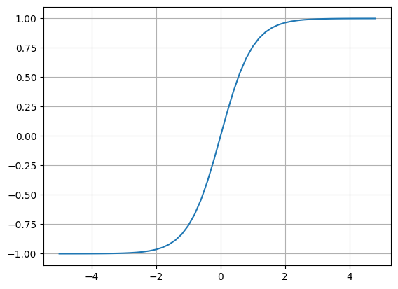
Tanh (Hyperbolic Tangent)

The hyperbolic tangent function squashes inputs into the range $[-1, 1]$ .

\tanh(x) = \frac{e^{2x} - 1}{e^{2x} + 1}

Zero-centered: The output can be positive or negative.
Smooth gradient: Good for backpropagation.

Numpy has the tanh function and we can visualize the function in python. This allows us to see that tanh is a compression function applied to the dot product of inputs $x_i$ and $w_i$ . When the input is negative we see the output approaches -1 and when positive it approaches +1.

plt.plot(np.arange(-5, 5, 0.2), np.tanh(np.arange(-5, 5, 0.2))); plt.grid();

Expressing The Neuron As A Mathematical Function

We can now express the simple neural network as a mathematical expression. We add intermediate Value objects to breakdown the expression. After the value n is computed it is passed to an activation function i.e. tanh to constrain the output to values between -1 and +1. We have to implement a tanh method for the Value class so that it can take the n as input and give the output o.

Above we see that $\tanh$ can be calculated using the $e^{2x}$ . However it is not necessary to implement an exponent method for the Value class we need only implement operations that are differentiable in the backpropagation process. Therefore we implement the tanh method for the Value class.

# inputs x1, x2 to the neuron
x1 = Value(2.0, label='x1')
x2 = Value(0, label='x2')

# weights w1, w2 to the neuron
w1 = Value(-3.0, label='w1')
w2 = Value(1.0, label='w2')

# bias to the neuron set to special value 6.8813735870195432 to get nice numbers later in backpropagation
b = Value(6.8813735870195432, label='b')

# x1*w1 + x2*w2 + b
x1w1 = x1*w1; x1w1.label='x1w1'
x2w2 = x2*w2; x2w2.label='x2w2'

x1w1x2w2 = x1w1 + x2w2; x1w1x2w2.label='x1w1 + x2w2'

n = x1w1x2w2 + b; n.label = 'n'

o = n.tanh(); o.label = 'o'

draw_dot(o)

Calculating Gradients For Nodes Of the Neural Network Expression

This part is manual calculation of gradients for each of the nodes in the above mathematical expression. The diagram above did not have any gradients assigned. The gradients for each of the nodes is computed.

$do/do$

The gradient of $o$ w.r.t $o$ is 1

o.grad = 1.0

$do/dn$

The gradient of $o$ w.r.t $n$ is the derivative of $tanh$ has many different formulae but we choose the most accessible i.e.

\frac{d}{dx} \tanh(x) = 1 - \tanh^2(x)

Since $o = tanh(n)$ we can represent the derivative w.r.t n as $\frac{d}{dn} \tanh(n) = 1 - \tanh^2(n) = 1 - o^2$

Here’s we get 0.5 which is because we set the special value of 6.8813735870195432 above for the bias b

n.grad = 1 - o.data**2

$do/db$ and $do/d(x1w1+x2w2)$

The gradient here can be routed from the output gradient as the operation is addition and the local derivative is 1 for each of the nodes. This stems from our initial manual backpropagation exercise above. So the gradients will be equal to the output gradient which was calculated above i.e. 0.5

x1w1x2w2.grad = n.grad
b.grad = n.grad

$do/dx1w1$ and $do/dx2w2$

Again here gradient is routed from the output for each of the nodes. The gradient for each node is 0.5

x1w1.grad = x1w1x2w2.grad
x2w2.grad = x1w1x2w2.grad

$do/dx1$ and $do/dw1$ and $do/dx2$ and $do/dw2$

Since the output for these nodes is through the multiplication operation the local derivative is the multiplication of other nodes contributing to the multiplication. This means we have to multiply the data of the node with the gradient of the output. Again this is explained in the simple exercise above.

x1.grad = w1.data * x1w1.grad
w1.grad = x1.data * x1w1.grad

x2.grad = w2.data * x2w2.grad
w2.grad = x2.data * x2w2.grad

draw_dot(o)

Part 5: Automating Backpropagation

We automate the backpropagation process. First we modify the class Value and define a _backward method. This will store the backpropagation function. For a leaf node this is a NOP and is implemented as an anonymous function. We have added this method and assigned it self._backward = lambda : None.

Updating `init`

Nodes that you create manually (like inputs $x$ or weights $w$ ) aren’t the result of a mathematical operation. Therefore, they don’t have a “backward” logic to perform—there is nowhere else for them to pass the gradient. By default, their _backward does nothing.

When you automate backpropagation, you want to loop through every node in your graph and call its backward function:

for node in reversed(topo):
    node._backward()

If leaf nodes didn’t have a function assigned to _backward, the code would crash. By using lambda: None, you ensure that every single node has a function you can safely call, even if that function is just an empty placeholder.

Python Concepts Learned:

lambda: This keyword creates an anonymous function ( a function without a name). The : separates the arguments from the return value

Updating `add`

We create a closure named _backward within __add__ to code the backpropagation operation for an addition operation. From our previous manual backpropagation exercise this routes the gradient to the output node to the children nodes because the local derivative of an addition operation is 1 and with the chain rule we multiply the output gradient with the local gradient. This gives us the following implementation for the closure

def _backward():
    self.grad = 1 * out.grad
    other.grad = 1 * out.grad

Updating `mul`

We create a closure named _backward within __mul__ to code the backpropagation operation for a multiplication operation. From our previous manual backpropagation exercise this multiplies the gradient to the output node to the children nodes because the local derivative of an addition operation is the multiplication of other noded and with the chain rule we multiply the output gradient with the local gradient. This gives us the following implementation for the closure

def _backward():
    self.grad = other.data * out.grad
    other.grad = self.data * out.grad

Updating `tanh`

In the case of tanh we define a local variable t = (math.exp(2*self.data) - 1)/(math.exp(2*self.data) + 1). So we use that in the _backward definition.

t = (math.exp(2*self.data) - 1)/(math.exp(2*self.data) + 1)

def _backward():
    self.grad = (1 - t**2) * out.grad

Calculating Gradients For Each Operation Using `_backward` Methods

Having implemented the _backward methods for each of the operations we can redo the calculation of gradients. We will repeat the step of initializing the Value objects of the neural network and then proceed to use the new methods created.

# inputs x1, x2 to the neuron
x1 = Value(2.0, label='x1')
x2 = Value(0, label='x2')

# weights w1, w2 to the neuron
w1 = Value(-3.0, label='w1')
w2 = Value(1.0, label='w2')

# bias to the neuron set to special value 6.8813735870195432 to get nice numbers later in backpropagation
b = Value(6.8813735870195432, label='b')

# x1*w1 + x2*w2 + b
x1w1 = x1*w1; x1w1.label='x1w1'
x2w2 = x2*w2; x2w2.label='x2w2'

x1w1x2w2 = x1w1 + x2w2; x1w1x2w2.label='x1w1 + x2w2'

n = x1w1x2w2 + b; n.label = 'n'

o = n.tanh(); o.label = 'o'

# Uncomment draw_dot to verify all gradients are 0
# draw_dot(o)

The output gradient is the base case so it should be initialized to 1

o.grad = 1

o._backward()

n._backward()

b._backward()

x1w1x2w2._backward()

x1w1._backward()

x2w2._backward()

draw_dot(o)

Implementing Backpropagation For The Whole Neural Network

We’ve been able to automate the backpropagation work for each operation. Now it’s time to automate the flow of backpropagation and for this we use topological sort. This is important because we need to iterate through all the nodes in a manner where dependencies are preserved. This is essential for the _backward function to work. We cannot compute _backward for a node if we don’t have the output gradient.

Topological Sort

Topological sort is the algorithm that is at the heart of sequencing the nodes for backpropagation. We test out the algorithm with a simple function build_topo. The order of topo has to be reversed for backpropogation

visited = set()
topo = []

def build_topo(v):
    if v not in visited:
        visited.add(v)
        for child in v._prev:
            build_topo(child)
        topo.append(v)

build_topo(o)
topo

[Value(Data=6.881373587019543),
 Value(Data=-3.0),
 Value(Data=2.0),
 Value(Data=-6.0),
 Value(Data=0),
 Value(Data=1.0),
 Value(Data=0.0),
 Value(Data=-6.0),
 Value(Data=0.8813735870195432),
 Value(Data=0.7071067811865476)]

Implementing The `backward` Method For The Value Class

We add this functionality to a backward class where we call _backward for each of the Value objects in reverse order after the topological sort. We can see the following in the Value class definition:

    def backward(self):
        visited = set()
        topo = []
        def build_topo(v):
            if v not in visited:
                visited.add(v)
                for child in v._prev:
                    build_topo(child)
                topo.append(v)

        build_topo(self)

        self.grad = 1

        for node in reversed(topo):
            node._backward()

With this function in place we can call backward method on the Value object o. Visualizing the expression we can see that we have automated the process of backpropagation which we were doing manually previously.

# inputs x1, x2 to the neuron
x1 = Value(2.0, label='x1')
x2 = Value(0, label='x2')

# weights w1, w2 to the neuron
w1 = Value(-3.0, label='w1')
w2 = Value(1.0, label='w2')

# bias to the neuron set to special value 6.8813735870195432 to get nice numbers later in backpropagation
b = Value(6.8813735870195432, label='b')

# x1*w1 + x2*w2 + b
x1w1 = x1*w1; x1w1.label='x1w1'
x2w2 = x2*w2; x2w2.label='x2w2'

x1w1x2w2 = x1w1 + x2w2; x1w1x2w2.label='x1w1 + x2w2'

n = x1w1x2w2 + b; n.label = 'n'

o = n.tanh(); o.label = 'o'

o.backward()

draw_dot(o)

Fixing A BAD Bug

The joy of getting backpropagation implemented is short lived. We’re taken through a couple of use cases where our implementation falls short. These are bugs that will probably break the implementation for more complicated neural networks.

Consider the simplest case of a reused variable:

a = Value(3.0)
b = a + a  # 'a' is reused here

Mathematically, $b = 2a$ , so the derivative $\frac{db}{da}$ should be 2. However, in the _backward logic for addition we see that the gradient for self.grad and other.grad is implemented with simple assignment (=):

# BUGGY IMPLEMENTATION
def _backward():
    self.grad = 1.0 * out.grad   # Path 1: sets a.grad to 1.0
    other.grad = 1.0 * out.grad  # Path 2: overwrites a.grad to 1.0

Because self and other are both pointing to the same object (a), the second line wipes out the work of the first line. The result is a.grad = 1.0, which is wrong.

This bug is a direct violation of the Multivariate Chain Rule in calculus.

If a variable $x$ influences an output $L$ through multiple independent paths (let’s call them $u$ and $v$ ), the total change in $L$ is the sum of the changes flowing back through all paths:

\frac{dL}{dx} = \frac{\partial L}{\partial u} \frac{du}{dx} + \frac{\partial L}{\partial v} \frac{dv}{dx}

In our $b = a + a$ example:

$u = a$ (first input)
$v = a$ (second input)
The total derivative is $1 + 1 = 2$ .

To solve this, we must change our gradient updates from assignment (=) to accumulation (+=). This ensures that every time a variable is used in the graph, its contribution to the final gradient is added to its existing total.

Corrected Implementation:

# FIXED IMPLEMENTATION
def _backward():
    self.grad += 1.0 * out.grad   # Accumulate contribution from Path 1
    other.grad += 1.0 * out.grad  # Accumulate contribution from Path 2

a = Value(1.0, label='a')
b = a + a; b.label = 'b'
b.backward()
print(a.grad) # We should see 2.0
draw_dot(b) # We should see grad as 2.0

2.0

Karpathy gives another example to demonstrate why we have to accumulate the gradients if a value is used in multiple paths.

a = Value(-2.0, label='a')
b = Value(3.0, label='b')
d = a + b
e = a * b
f = e * d
f.backward()
draw_dot(f)

Part 6: Expanding tanh And Adding More Operations To Value Class

In the previous sections, we implemented tanh as a single, atomic operation. However, tanh is actually a composite function:

\tanh(x) = \frac{e^{2x} - 1}{e^{2x} + 1}

To make our engine more powerful, we want to break this down into its fundamental components. This requires adding support for exponentiation, powers, division, and subtraction to our Value class.

The Power Operator (`pow`)

The power operator is critical for handling non-linearities and is the mathematical foundation for division ( $1/x$ is $x^{-1}$ ).

def __pow__(self, other):
    assert isinstance(other, (int, float)), "only supporting int/float powers for now"
    out = Value(self.data**other, (self,), f'**{other}')

    def _backward():
        self.grad += (other * self.data**(other - 1)) * out.grad
    out._backward = _backward

    return out

The Power Rule: We apply the standard calculus rule $\frac{d}{dx}x^n = nx^{n-1}$ .
Chain Rule Integration: The local derivative is multiplied by out.grad to propagate the gradient correctly back to self.

The Exponential Function (`exp`)

To handle the $e^x$ terms in the $\tanh$ formula, we implement a specific exp method.

def exp(self):
    x = self.data
    out = Value(math.exp(x), (self, ), 'exp')
    
    def _backward():
        self.grad += out.data * out.grad
    out._backward = _backward
    
    return out

Self-Derivative: The derivative of $e^x$ is simply $e^x$ .
Efficiency: Since $e^x$ is already calculated and stored in out.data, the backward pass requires no extra heavy math.

Subtraction and Division

Instead of writing new derivative logic for these operations, we can define them as combinations of addition, multiplication, and power.

def __neg__(self): # -self
    return self * -1

def __sub__(self, other): # self - other
    return self + (-other)

def __truediv__(self, other): # self / other
    return self * (other**-1)

Negation: Implemented as multiplication by the constant -1.
Subtraction: Implemented as adding a negative value ( $a - b \equiv a + (-b)$ ).
Division: Implemented as multiplying by a reciprocal ( $a / b \equiv a \cdot b^{-1}$ ), which leverages our __pow__ method.

Reflected Operators and Constants

To ensure our class handles operations like 2 * a or 1 + a (where the Value object is on the right), we implement “reflected” methods.

def __radd__(self, other): # other + self
    return self + other

def __rmul__(self, other): # other * self
    return self * other

Reflected Logic: These methods are called by Python when the left-hand operand does not support the operation with a Value object.
Seamless Integration: This allows the Value class to interact with native Python types (int, float) just like a real number would.

Verification: The Composite Tanh

Let’s setup the neural network expression again. We’ll repeat the expression using tanh first to check the weights then we will subsitute it with a formula to calculate tanh. When we run the expression using tanh we get the following output Value as 0.707107 due to the expression. We get the gradients of x1, w1, x2 and w2 as -1.5, 1.0, 0.5 and 0.0.

# inputs x1, x2 to the neuron
x1 = Value(2.0, label='x1')
x2 = Value(0, label='x2')

# weights w1, w2 to the neuron
w1 = Value(-3.0, label='w1')
w2 = Value(1.0, label='w2')

# bias to the neuron set to special value 6.8813735870195432 to get nice numbers later in backpropagation
b = Value(6.8813735870195432, label='b')

# x1*w1 + x2*w2 + b
x1w1 = x1*w1; x1w1.label='x1w1'
x2w2 = x2*w2; x2w2.label='x2w2'

x1w1x2w2 = x1w1 + x2w2; x1w1x2w2.label='x1w1 + x2w2'

n = x1w1x2w2 + b; n.label = 'n'

o = n.tanh()

o.backward()

draw_dot(o)

We can now represent the same neuron logic using these fundamental building blocks:

# Composite tanh calculation
e = (2*n).exp()
o = (e - 1) / (e + 1)

o.backward()

By breaking tanh into exp, sub, and div, we can see the gradients flow through every sub-operation in the graph, confirming our autograd engine handles nested functions perfectly.

# inputs x1, x2 to the neuron
x1 = Value(2.0, label='x1')
x2 = Value(0, label='x2')

# weights w1, w2 to the neuron
w1 = Value(-3.0, label='w1')
w2 = Value(1.0, label='w2')

# bias to the neuron set to special value 6.8813735870195432 to get nice numbers later in backpropagation
b = Value(6.8813735870195432, label='b')

# x1*w1 + x2*w2 + b
x1w1 = x1*w1; x1w1.label='x1w1'
x2w2 = x2*w2; x2w2.label='x2w2'

x1w1x2w2 = x1w1 + x2w2; x1w1x2w2.label='x1w1 + x2w2'

n = x1w1x2w2 + b; n.label = 'n'

# Composite tanh calculation
e = (2*n).exp()
o = (e - 1)/(e + 1)

o.backward()

draw_dot(o)

Part 7: Comparison with Pytorch

In this section we explore what the corresponding implementation would look like in Pytorch. To do this we implement the neural network with pytorch. The Tensor class of Pytorch is the equivalent of the Value class we have implemented.

import torch

x1 = torch.Tensor([2.0]).double(); x1.requires_grad = True;
x2 = torch.Tensor([0.0]).double(); x2.requires_grad = True;
w1 = torch.Tensor([-3.0]).double(); w1.requires_grad = True;
w2 = torch.Tensor([1.0]).double(); w2.requires_grad = True;

b = torch.Tensor([6.8813735870195432]); b.requires_grad = True;

n = x1*w1 + x2*w2 + b

o = torch.tanh(n)

print(o.item())
o.backward()

print('---')
print(x1.grad.item())
print(x2.grad.item())

print(w1.grad.item())
print(w2.grad.item())

0.7071066904050358
---
-1.5000003851533106
0.5000001283844369
1.0000002567688737
0.0

We see that the gradients are the same as that computed with our implementation of micrograd.

The micrograd implementation works on scalars whereas if we observe Pytorch is designed to handle Tensors which are multi-dimensional arrays. This allows it to run operations across a group of values on a GPU which is designed for this type of computation.

Pytorch doesn’t compute gradients for leaf nodes and so we need to explicitly set the requires_grad for each of the values to True as they are leaf nodes in the expression.

There is API consistency observed between the Pytorch and micrograd libraries. For instance the backward method is the same and gradients are stored in .grad just like the Value class we defined.

Part 8: Building out the neural network library and using it to build out a two layer multilayer perceptron

After trying out the pytorch library and getting a sense of the API and its similarities with micrograd while performing the autograd operation we now attempt to build out neural network modules in the same design of pytorch.

class Neuron:
    def __init__(self, nin):
        self.w = [Value(random.uniform(-1, 1)) for _ in range(nin)]
        self.b = Value(random.uniform(-1, 1))

    def __call__(self, x):
        # w*x + b
        act = sum((wi*xi for wi,xi in zip(self.w, x)), self.b)
        out = act.tanh()
        return out

    def parameters(self):
        return self.w + [self.b]

x = [2.0, 3.0]
n = Neuron(2)
n(x)

Value(Data=-0.2829908053190328)

The above is our model of a neuron. In the previous sections we focussed on understanding the mechanics of autogradient using mathematical expressions. We see that the value returned changes everytime we run it because the weights of the neuron are initialized using random numbers.

The dunder method __call__ is used to give the Neuron class a function like propery whereby after initialization the neuron can be used to compute the output based on the input as shown as n(x) above.

class Layer:
    def __init__(self, nin, nout):
        self.neurons = [Neuron(nin) for _ in range(nout)]

    def __call__(self, x):
        outs = [n(x) for n in self.neurons]
        return outs[0] if len(outs) == 1 else outs

    def parameters(self):
        return [p for neuron in self.neurons for p in neuron.parameters()]

x = [21.0, 22.0]
l = Layer(3, 4)
l(x)

[Value(Data=0.9999806398424194),
 Value(Data=0.9984223312594778),
 Value(Data=-0.9930973730871919),
 Value(Data=-0.9999999010535582)]

The above is our model of a layer of the neural network. It takes the number of inputs and outputs as arguments. The neurons of the layer are initialized based on the number of outputs. For each output a neuron with nin inputs is initialized and assigned to the neurons of the layer. The __call__ method is defined to build the list of computed neuron values if this list is of size 1 then the first element is returned.

class MLP:
    def __init__(self, nin, nouts):
        sz = [nin] + nouts
        self.layers = [Layer(sz[i], sz[i + 1]) for i in range(len(nouts))]

    def __call__(self, x):
        for layer in self.layers:
            x = layer(x)
        return x

    def parameters(self):
        return [p for layer in self.layers for p in layer.parameters()]

We define the multi-layer perceptron model above. The initialization takes the number of inputs as one argument and the list of outputs for each of the layers as the second argument. In the __init__ method sz is a list of sizes inclusive of the inputs. It combines your input count with all your layer output counts into a single list that represents every stage of the network.

Suppose we require a MLP that takes 3 inputs, has 2 hidden layers of 4 neurons and 1 final output we would pass nin = 3 and nouts = [4, 4, 1]. The line sz = [nin] + nouts results in sz = [3, 4, 4, 1]

With the list [3, 4, 4, 1], we can easily loop through it to create the pairs:

Layer 1: Inputs = 3, Outputs = 4 (takes sz[0] and sz[1])
Layer 2: Inputs = 3, Outputs = 4 (takes sz[1] and sz[2])
Layer 3: Inputs = 3, Outputs = 4 (takes sz[2] and sz[3])

mlp = MLP(3, [4, 4, 1])

mlp(x)

Value(Data=0.007119412666099561)

We can also visualize the expression using draw_dot but it would be complex to analyze

draw_dot(mlp(x))

Part 9: Creating a dataset for training

With our class definitions in place we will now create a dataset of inputs and expected values. This dataset will represent the range of data inputs and expected outputs that we desire our neural network to approximate. We have the input xs which is a list of 4 lists of 3 values each as the MLP we have defined above has 3 inputs. And the output is also a list where each value corresponds to the ground truth or expected output of the MLP. The neural network is simple binary classifier which gives an output of either 1.0 or -1.0 based on the input.

xs = [
    [2.0, 3.0, -1.0],
    [3.0, -1.0, 0.5],
    [0.5, 1.0, 1.0],
    [1.0, 1.0, -1.0]
]

ys = [
    1.0,
    -1.0,
    -1.0,
    1.0
]

ypred = [mlp(x) for x in xs]

ypred # Print values to check proximity to ys values

[Value(Data=-0.28831424353406127),
 Value(Data=0.323450361187395),
 Value(Data=-0.0997348332221718),
 Value(Data=-0.2713241381880621)]

The output values will be either closer to 1.0 or -1.0 depending on the value of the randomized weights which were initialized when the neuron was constructed. To guage the effectiveness of the MLP we would need to define a value which measures the difference in predicted output from the ground truth. This value can be used as a guide to tune the weights of the neural network in order to better approximate the data set. Andrej Karpathy describes it best:

How do we tune the neural network to best predict the desired outputs. The trick used in deep learning is to calculate a single number that somehow measures total performance of the neural network. We call this single number the loss.

One approach would be to compute the difference between the predicted and expected values. This however would result in negative values. To counter this we can either take the absolute of the difference or square the difference. We use the square here.

loss = [(yout - ygt)**2 for ygt, yout in zip(ys, ypred)]

loss # Print values to confirm loss is 0 for values predicted correctly

[Value(Data=1.6597535900927407),
 Value(Data=1.751520858527046),
 Value(Data=0.8104773705135108),
 Value(Data=1.616265064339619)]

If we check the loss components we get values that are positive and greater than 0 or values that are 0. The values that are 0 indicate that the MLP is able to predict the output based on the desired ground truth output. The values that are not 0 indicate that the MLP is not able to predict the output correctly.

In order to calculate a single number we sum the values of all losses to get a single loss value. This value will be close to 0 when the MLP is able to predict outputs which match the ground truth dataset. The greater this value the worse off the neural network is at predicting the output as per the desired data set.

loss = sum((yout - ygt)**2 for ygt, yout in zip(ys, ypred))

loss

Value(Data=5.838016883472917)

If we now run the backward method on the loss value we will be able to see the gradients for all the values of the mathematical expression that makes up the loss. We check the value of the gradient for the weight of the first neuron of the first layer of the MLP.

loss.backward()

mlp.layers[0].neurons[0].w[0].grad

-1.7420496127450584

To understand how this gradient can be used to adjust the corresponding weight of the neuron of the layer of the MLP we reflect on this statement by Andrej Karpathy:

Because the gradient is negative we see that its influence on the loss of the neural network is also negative. Slightly increasing this particular weight of this neuron of this layer will make the loss go down.

If we were to visualize the graph for the loss expression we would get an immensely complex graph as the loss function is a summation of losses for each of the predictions of the neural network. It depicts 4 forward passes of the MLP for each of the inputs of the data set coupled with the computation of loss for each of the inputs and summed up to give the final mean square loss value.

draw_dot(loss)

Part 10: Gradient Descent

In order to tune the MLP we have to perform an operation called gradient descent. This is a procedure which modifies the gradients of all the parameters of the MLP in order to achieve a negligible loss.

Collecting Parameters

The parameters of the neural network include weights and biases of each of the neurons across all the layers of the network. These are the value which when nudged in the right direction allow the MLP to achieve its approximation of the data set which is used for training. We define a parameters method for each of the modules similar to what is present in Pytorch to get the list of parameters across all neurons in the neural network.

For the Neuron class the parameters is defined as a concatenation of the weights which is a list with a list formed with the biases. The number of parameters for each neuron will be the sum of number of inputs (corresponding to the number of weights) plus the bias value i.e. nin + 1.

# definition of method parameters in class Neuron
    def parameters(self):
        return self.w + [self.b]

ntemp = Neuron(3)
ntemp.parameters()
len(ntemp.parameters()) # This should be 4 which is number of inputs (corresponding to the number of weights)

For the Layers class the parameters is defined as the concatenation of all the parameters of all the neurons. The number of parameters for each layer will be the number of neurons in that layer multiplied by the number of parameters in a layer.

    # definition of method parameters in class Layers
        def parameters(self):
            return [p for neuron in self.neurons for p in neuron.parameters()]

Python Concepts Learned:

We can use list comprehension to simplify the implementation of parameters.

layertemp = Layer(3, 4)
layertemp.parameters()
len(layertemp.parameters()) # This should be 16 as the number of parameters/neuron is 4 and number of neurons is 4

For the MLP class the parameters is defined as the concatenation of all the parameters of all the layers. The number of parameters for the MLP is the number of layers multiplied by the number of layers in a MLP.

    # definition of method parameters in class MLP
        def parameters(self):
            return [p for layer in self.layers for p in layer.parameters()]

mlptemp = MLP(3, [4, 4, 1])
mlptemp.parameters()
len(mlptemp.parameters()) # This should be 41 ((3+1) x 4 + (4+1) x 4 + (4+1) x 1)

mlptemp.parameters()

[Value(Data=-0.05123286423177231),
 Value(Data=-0.5516558347104326),
 Value(Data=0.4298889942579578),
 Value(Data=-0.4013941291718779),
 Value(Data=-0.5376348174590795),
 Value(Data=0.9922452976338012),
 Value(Data=0.7640396429970322),
 Value(Data=-0.8355503853699362),
 Value(Data=-0.44287158487507483),
 Value(Data=0.3480447219734337),
 Value(Data=0.15972928011029852),
 Value(Data=-0.8026188606247451),
 Value(Data=-0.5657217935999479),
 Value(Data=-0.4414344169120408),
 Value(Data=-0.2548455935029299),
 Value(Data=-0.1505759141400922),
 Value(Data=0.8000433484234859),
 Value(Data=-0.6373304636063479),
 Value(Data=0.7600296798535993),
 Value(Data=-0.2516629795328158),
 Value(Data=0.6949269163904792),
 Value(Data=-0.476972312667431),
 Value(Data=0.12355534813865865),
 Value(Data=0.7654419807806421),
 Value(Data=0.22941516156045938),
 Value(Data=-0.7336415442362707),
 Value(Data=-0.6927777806295639),
 Value(Data=0.6064936829205212),
 Value(Data=-0.7378573011870964),
 Value(Data=-0.5819286108975674),
 Value(Data=-0.10216131582938726),
 Value(Data=-0.4736152362124768),
 Value(Data=-0.05171111249428839),
 Value(Data=-0.4673126125192677),
 Value(Data=0.67073606318594),
 Value(Data=-0.7598980821867987),
 Value(Data=0.07799944037642792),
 Value(Data=0.5175052209034297),
 Value(Data=0.15883830241646013),
 Value(Data=-0.9346502191117401),
 Value(Data=0.20787035156982459)]

Manual Gradient Descent

We can manually see the effect of gradient descent by repeating the following steps in a loop. The step size step can be changed to increase the speed of gradient descent. As we iterate through these steps we should be able to see our MLP giving a prediction that is closer to the ground truth. We use the same dataset we created above with xs and ys values. The steps to be followed in a loop are:

Forward pass
Compute loss
Zero grad
Backpropagation of loss
Tune weights based on gradients

During the lecture Karpathy increases the step size/learning rate to increase the speed of training. In my experiement I keep it fixed at 0.01 as this is sufficient to gain an intuitive understanding of the training process. Setting a learning rate that is too high leads to overstepping which briefly takes the loss higher before settling to a very low value

Setting the learning rate is apparently an art where setting it too high may lead to over stepping whereas setting it too low would result in an undesirably long training time.

# Initialize the multi-layer perceptron. Make sure to run this once. 
mlp = MLP(3, [4, 4, 1])

The following steps are to be run in a loop until the loss becomes negligible. At this point we should see the ypred should be approximately equal to ys.

# Step 1: Forward pass
ypred = [mlp(x) for x in xs]
ypred

[Value(Data=-0.8680141339553723),
 Value(Data=-0.05540848615480571),
 Value(Data=-0.7226046752582078),
 Value(Data=-0.806551534758723)]

# Step 2: Calculate the loss
loss = sum((yout - ygt)**2 for ygt, yout in zip(ys, ypred))
loss

Value(Data=7.722306546613096)

# Step 3: Zero grad
for p in mlp.parameters():
    p.grad = 0.0

# Step 4: Backpropagation
loss.backward()

# Step 5: Adjust weights
step = 0.01
for p in mlp.parameters():
    p.data += -step * p.grad

# Iterate from Step 1 till loss is minimal

The data that is modified is the value of the weight of the neuron. This is modified based on the gradient of the neuron.

mlp.layers[0].neurons[0].w[0].data

0.10114679009090354

mlp.layers[0].neurons[0].w[0].grad

-0.22611309264741572

Another Bad Bug

In the lecture Karpathy mentions that there is a common bug which is to not do a zero grad operation. This is basically resetting all the gradients to 0.0 before the backpropagation step. The effect of this is that the gradients keep accumulating across different iterations. In the first pass the gradient is reset because of the construction operation of the neuron. This is corrected and shown as step 3 in the manual gradient descent section above

Implementing a training loop

We can now wrap the manual steps in a training loop to automate the iterative process. We print the loss on each iteration to track it’s descent and once sufficiently low we can see that our prediction matches the ground truth of the data set

mlp = MLP(3, [4, 4, 1])
step = 0.01
nsteps = 1000

for k in range(nsteps):
    # Step 1: Forward pass
    ypred = [mlp(x) for x in xs]

    # Step 2: Calculate the loss
    loss = sum((yout - ygt)**2 for ygt, yout in zip(ys, ypred))

    # Step 3: Zero grad
    for p in mlp.parameters():
        p.grad = 0.0

    # Step 4: Backpropagation
    loss.backward()

    # Step 5: Adjust weights

    for p in mlp.parameters():
        p.data += -step * p.grad

    print(k, loss.data)

0 5.359211953467817
1 4.080862093346827
2 3.210459800500157
3 2.6046199367895695
4 2.147040340927046
5 1.7983871293798683
6 1.5306179935039363
7 1.321649001159321
8 1.1555258242292177
9 1.0211287248368857
10 0.9106935977225753
11 0.8187075303184452
12 0.741174432838776
13 0.6751385820081658
14 0.6183730980952737
15 0.5691724094261055
16 0.5262109941382893
17 0.4884451935042681
18 0.45504362539992693
19 0.42533699199936625
20 0.39878129849016986
21 0.37493051210988726
22 0.3534159745158864
23 0.3339307163984467
24 0.3162173781705878
25 0.30005881558622005
26 0.28527072674546705
27 0.27169581656165936
28 0.259199141723758
29 0.2476643700607677
30 0.23699075401486175
31 0.22709066608780265
32 0.21788757972315576
33 0.20931440564545117
34 0.20131211366458704
35 0.19382858511825724
36 0.1868176527189901
37 0.1802382935004647
38 0.17405394748012692
39 0.168231940057128
40 0.16274299040612128
41 0.1575607914772487
42 0.15266164987294156
43 0.14802417599608336
44 0.14362901656837868
45 0.13945862299198097
46 0.1354970501406153
47 0.13172978107218639
48 0.12814357389497505
49 0.1247263276267638
50 0.12146696438641819
51 0.11835532567099148
52 0.11538208081460372
53 0.11253864601110211
54 0.10981711252128132
55 0.10721018288558905
56 0.10471111413154088
57 0.10231366710702143
58 0.10001206119072717
59 0.09780093373286905
60 0.09567530366590292
61 0.09363053879895594
62 0.0916623263728114
63 0.08976664650648308
64 0.08793974821295708
65 0.08617812770176922
66 0.08447850872069487
67 0.082837824718768
68 0.0812532026388074
69 0.0797219481701788
70 0.07824153231215888
71 0.07680957911538937
72 0.07542385448388088
73 0.07408225593312855
74 0.07278280321139696
75 0.07152362970133162
76 0.0703029745279462
77 0.0691191753068717
78 0.06797066147367602
79 0.06685594814118583
80 0.06577363043716539
81 0.06472237827952139
82 0.06370093155047525
83 0.06270809563495275
84 0.061742737291827665
85 0.06080378082968388
86 0.05989020456146085
87 0.05900103751476612
88 0.05813535637680556
89 0.05729228265482294
90 0.05647098003468615
91 0.05567065192182523
92 0.054890539150140825
93 0.054129917845770495
94 0.053388097433752696
95 0.05266441877666197
96 0.05195825243522615
97 0.05126899704178647
98 0.05059607777822978
99 0.04993894495071684
100 0.049297072654166905
101 0.048669957520033
102 0.048057117541421945
103 0.04745809097009598
104 0.04687243528031945
105 0.04629972619491819
106 0.045739556769270884
107 0.04519153652929044
108 0.044655290659751545
109 0.04413045923959594
110 0.04361669652110278
111 0.043113670250041064
112 0.04262106102413599
113 0.0421385616873748
114 0.04166587675785848
115 0.04120272188707079
116 0.04074882334858643
117 0.04030391755438233
118 0.0398677505970446
119 0.039440077816279284
120 0.03902066338825127
121 0.038609279936369645
122 0.03820570816223778
123 0.03780973649556835
124 0.03742116076194655
125 0.037039783867397445
126 0.03666541549878292
127 0.03629787183911572
128 0.035936975296940274
129 0.03558255424898149
130 0.03523444279531518
131 0.03489248052636229
132 0.034556512301048864
133 0.034226388035521055
134 0.03390196250183605
135 0.03358309513608915
136 0.03326964985546969
137 0.03296149488376794
138 0.03265850258488535
139 0.0323605493039261
140 0.032067515215474005
141 0.03177928417868167
142 0.031495743598819605
143 0.031216784294956487
144 0.030942300373456157
145 0.030672189107000137
146 0.03040635081885646
147 0.03014468877213449
148 0.029887109063778547
149 0.029633520523067544
150 0.029383834614400056
151 0.02913796534415767
152 0.028895829171448863
153 0.028657344922549233
154 0.028422433708860412
155 0.02819101884822208
156 0.027963025789419945
157 0.027738382039739898
158 0.027517017095426855
159 0.02729886237491526
160 0.02708385115470307
161 0.026871918507750003
162 0.026663001244285105
163 0.026457037854914985
164 0.02625396845593116
165 0.0260537347367172
166 0.025856279909163917
167 0.025661548659004104
168 0.025469487098983105
169 0.025280042723785635
170 0.025093164366642585
171 0.024908802157546477
172 0.024726907483006516
173 0.024547432947278153
174 0.024370332335004706
175 0.02419556057521247
176 0.024023073706601776
177 0.023852828844082075
178 0.02368478414649756
179 0.023518898785496626
180 0.023355132915497078
181 0.023193447644703245
182 0.02303380500713285
183 0.022876167935612503
184 0.022720500235703673
185 0.022566766560522332
186 0.022414932386416335
187 0.022264963989467562
188 0.02211682842278675
189 0.02197049349456909
190 0.021825927746882814
191 0.021683100435161334
192 0.021541981508372512
193 0.021402541589839688
194 0.021264751958688866
195 0.02112858453189971
196 0.020994011846936493
197 0.02086100704493843
198 0.020729543854447897
199 0.020599596575657277
200 0.020471140065155078
201 0.020344149721153088
202 0.020218601469177293
203 0.020094471748205327
204 0.019971737497235426
205 0.019850376142269883
206 0.01973036558369972
207 0.01961168418407542
208 0.019494310756250285
209 0.019378224551884135
210 0.019263405250292874
211 0.01914983294763421
212 0.0190374881464162
213 0.018926351745317704
214 0.018816405029311707
215 0.01870762966007805
216 0.01860000766669916
217 0.018493521436626276
218 0.018388153706909625
219 0.018283887555681316
220 0.018180706393884534
221 0.01807859395723925
222 0.017977534298437965
223 0.01787751177956288
224 0.017778511064717863
225 0.01768051711286802
226 0.017583515170879756
227 0.017487490766755813
228 0.017392429703057797
229 0.017298318050511005
230 0.017205142141785743
231 0.017112888565448715
232 0.017021544160080247
233 0.01693109600855131
234 0.01684153143245527
235 0.016752837986690534
236 0.016665003454187872
237 0.016578015840779406
238 0.016491863370204005
239 0.01640653447924491
240 0.01632201781299609
241 0.016238302220253107
242 0.01615537674902425
243 0.016073230642159465
244 0.015991853333091954
245 0.015911234441690826
246 0.015831363770219865
247 0.015752231299400406
248 0.015673827184574662
249 0.015596141751966799
250 0.015519165495038699
251 0.015442889070937701
252 0.015367303297033804
253 0.015292399147543607
254 0.015218167750238184
255 0.01514460038323329
256 0.015071688471858472
257 0.014999423585603784
258 0.01492779743514123
259 0.014856801869419255
260 0.014786428872828106
261 0.014716670562433538
262 0.014647519185278148
263 0.014578967115747018
264 0.014511006852997256
265 0.014443631018448257
266 0.014376832353332474
267 0.014310603716303855
268 0.014244938081102772
269 0.014179828534276403
270 0.014115268272952092
271 0.014051250602663112
272 0.01398776893522482
273 0.013924816786660375
274 0.013862387775174036
275 0.013800475619171703
276 0.013739074135326212
277 0.01367817723668747
278 0.013617778930835347
279 0.013557873318074396
280 0.013498454589669931
281 0.013439517026123256
282 0.013381054995485923
283 0.013323062951711907
284 0.013265535433046087
285 0.013208467060448939
286 0.01315185253605588
287 0.013095686641670747
288 0.01303996423729239
289 0.012984680259673378
290 0.01292982972091054
291 0.01287540770706577
292 0.012821409376817076
293 0.012767829960138578
294 0.012714664757009067
295 0.01266190913614831
296 0.012609558533780091
297 0.012557608452422129
298 0.01250605445970119
299 0.012454892187193839
300 0.012404117329291054
301 0.01235372564208719
302 0.01230371294229218
303 0.012254075106166265
304 0.01220480806847691
305 0.012155907821477668
306 0.012107370413908029
307 0.012059191950013697
308 0.012011368588587224
309 0.01196389654202829
310 0.011916772075423182
311 0.011869991505642774
312 0.011823551200459255
313 0.011777447577680253
314 0.011731677104300807
315 0.011686236295672028
316 0.011641121714686785
317 0.0115963299709814
318 0.011551857720153113
319 0.011507701662993614
320 0.011463858544737096
321 0.011420325154323556
322 0.011377098323676452
323 0.011334174926994425
324 0.011291551880057014
325 0.011249226139543874
326 0.011207194702367012
327 0.011165454605016327
328 0.011124002922917216
329 0.011082836769801253
330 0.011041953297088274
331 0.011001349693280676
332 0.010961023183369195
333 0.01092097102824978
334 0.01088119052415179
335 0.010841679002076873
336 0.010802433827248298
337 0.010763452398570898
338 0.010724732148100774
339 0.010686270540525292
340 0.010648065072652339
341 0.010610113272909564
342 0.010572412700852213
343 0.010534960946680787
344 0.01049775563076694
345 0.01046079440318854
346 0.010424074943272913
347 0.010387594959148538
348 0.01035135218730498
349 0.010315344392160563
350 0.010279569365638173
351 0.010244024926748422
352 0.010208708921180455
353 0.010173619220900085
354 0.010138753723754987
355 0.010104110353087222
356 0.010069687057352231
357 0.010035481809744907
358 0.010001492607832112
359 0.00996771747319182
360 0.009934154451058339
361 0.009900801609974148
362 0.009867657041447264
363 0.009834718859615205
364 0.00980198520091433
365 0.009769454223755044
366 0.009737124108202724
367 0.009704993055663979
368 0.009673059288578452
369 0.009641321050115727
370 0.00960977660387764
371 0.009578424233605474
372 0.009547262242892212
373 0.009516288954899655
374 0.009485502712080375
375 0.009454901875904259
376 0.00942448482658971
377 0.00939424996283937
378 0.009364195701580237
379 0.009334320477708115
380 0.009304622743836373
381 0.009275100970048744
382 0.009245753643656374
383 0.009216579268958771
384 0.009187576367008735
385 0.009158743475381148
386 0.009130079147945525
387 0.00910158195464232
388 0.009073250481262838
389 0.009045083329232761
390 0.00901707911539917
391 0.008989236471820976
392 0.008961554045562696
393 0.008934030498491858
394 0.008906664507079122
395 0.008879454762201967
396 0.00885239996895159
397 0.008825498846442504
398 0.00879875012762553
399 0.00877215255910348
400 0.008745704900950045
401 0.008719405926531186
402 0.008693254422329523
403 0.008667249187771623
404 0.008641389035057671
405 0.008615672788994135
406 0.008590099286828615
407 0.00856466737808775
408 0.008539375924417251
409 0.008514223799424537
410 0.008489209888523985
411 0.00846433308878414
412 0.008439592308777652
413 0.008414986468433291
414 0.008390514498890443
415 0.008366175342355401
416 0.00834196795196053
417 0.008317891291624606
418 0.008293944335916337
419 0.008270126069919035
420 0.008246435489097963
421 0.008222871599169197
422 0.008199433415970833
423 0.008176119965335864
424 0.008152930282967088
425 0.008129863414313805
426 0.008106918414450338
427 0.00808409434795643
428 0.008061390288799285
429 0.008038805320217609
430 0.008016338534606874
431 0.007993989033406689
432 0.007971755926989801
433 0.007949638334552422
434 0.007927635384006352
435 0.007905746211872773
436 0.007883969963177235
437 0.00786230579134664
438 0.007840752858107144
439 0.007819310333384144
440 0.00779797739520317
441 0.007776753229592435
442 0.007755637030486951
443 0.007734627999633528
444 0.007713725346497649
445 0.007692928288171285
446 0.007672236049282321
447 0.0076516478619049234
448 0.007631162965471501
449 0.007610780606685621
450 0.007590500039436474
451 0.007570320524714086
452 0.007550241330526198
453 0.007530261731815988
454 0.0075103810103809765
455 0.007490598454793294
456 0.00747091336032059
457 0.007451325028848646
458 0.007431832768804337
459 0.007412435895080444
460 0.007393133728960758
461 0.007373925598046782
462 0.007354810836185043
463 0.007335788783395627
464 0.007316858785801609
465 0.007298020195559423
466 0.007279272370790145
467 0.007260614675511864
468 0.007242046479572815
469 0.007223567158585409
470 0.0072051760938611886
471 0.007186872672346791
472 0.007168656286560416
473 0.007150526334529592
474 0.007132482219729369
475 0.007114523351021622
476 0.0070966491425949706
477 0.007078859013905576
478 0.007061152389618719
479 0.007043528699551226
480 0.007025987378614358
481 0.007008527866757867
482 0.006991149608914475
483 0.00697385205494513
484 0.006956634659585154
485 0.006939496882390862
486 0.0069224381876870356
487 0.006905458044514923
488 0.006888555926581042
489 0.006871731312206748
490 0.006854983684278081
491 0.006838312530196622
492 0.006821717341830806
493 0.006805197615467933
494 0.0067887528517666905
495 0.006772382555710389
496 0.006756086236560739
497 0.006739863407812201
498 0.006723713587147021
499 0.006707636296390627
500 0.006691631061467772
501 0.006675697412359235
502 0.006659834883058944
503 0.006644043011531591
504 0.006628321339671057
505 0.006612669413259127
506 0.0065970867819246885
507 0.006581572999103599
508 0.006566127621998958
509 0.006550750211541925
510 0.006535440332352948
511 0.006520197552703447
512 0.006505021444478133
513 0.006489911583137718
514 0.006474867547681859
515 0.006459888920612987
516 0.006444975287900173
517 0.006430126238943694
518 0.006415341366539898
519 0.006400620266846539
520 0.006385962539348526
521 0.006371367786824168
522 0.006356835615311635
523 0.006342365634076029
524 0.006327957455576671
525 0.006313610695435
526 0.006299324972402642
527 0.006285099908329912
528 0.006270935128134859
529 0.006256830259772379
530 0.006242784934204048
531 0.0062287987853679875
532 0.006214871450149276
533 0.006201002568350738
534 0.006187191782663876
535 0.0061734387386403935
536 0.006159743084663803
537 0.006146104471921663
538 0.0061325225543778505
539 0.006118996988745349
540 0.006105527434459203
541 0.006092113553649971
542 0.006078755011117401
543 0.006065451474304272
544 0.006052202613270823
545 0.0060390081006692145
546 0.006025867611718373
547 0.006012780824179276
548 0.0059997474183303085
549 0.005986767076942957
550 0.005973839485257811
551 0.00596096433096096
552 0.0059481413041604135
553 0.005935370097362863
554 0.00592265040545096
555 0.005909981925660493
556 0.005897364357558016
557 0.00588479740301869
558 0.005872280766204471
559 0.005859814153542295
560 0.005847397273702794
561 0.005835029837579075
562 0.0058227115582658116
563 0.005810442151038508
564 0.005798221333333103
565 0.005786048824725613
566 0.005773924346912215
567 0.005761847623689438
568 0.005749818380934587
569 0.005737836346586379
570 0.005725901250625767
571 0.005714012825057119
572 0.005702170803889393
573 0.0056903749231176064
574 0.0056786249207047045
575 0.0056669205365631765
576 0.0056552615125373806
577 0.005643647592385701
578 0.005632078521763086
579 0.005620554048203614
580 0.0056090739211035025
581 0.005597637891704047
582 0.005586245713074851
583 0.005574897140097221
584 0.005563591929447838
585 0.005552329839582406
586 0.005541110630719698
587 0.005529934064825571
588 0.005518799905597284
589 0.005507707918447978
590 0.005496657870491246
591 0.005485649530525874
592 0.005474682669020895
593 0.005463757058100623
594 0.005452872471529861
595 0.005442028684699405
596 0.0054312254746115805
597 0.005420462619865909
598 0.005409739900645095
599 0.005399057098700911
600 0.005388413997340441
601 0.005377810381412447
602 0.0053672460372937
603 0.005356720752875587
604 0.005346234317550996
605 0.00533578652220103
606 0.005325377159182099
607 0.005315006022313
608 0.005304672906862301
609 0.0052943776095356184
610 0.005284119928463289
611 0.005273899663187942
612 0.00526371661465233
613 0.00525357058518725
614 0.005243461378499634
615 0.005233388799660582
616 0.005223352655093793
617 0.005213352752563944
618 0.005203388901165123
619 0.005193460911309578
620 0.005183568594716459
621 0.00517371176440063
622 0.005163890234661681
623 0.005154103821073075
624 0.005144352340471283
625 0.005134635610945194
626 0.005124953451825379
627 0.005115305683673774
628 0.005105692128273241
629 0.005096112608617309
630 0.005086566948900066
631 0.005077054974506033
632 0.005067576512000207
633 0.005058131389118252
634 0.0050487194347567585
635 0.005039340478963398
636 0.005029994352927681
637 0.005020680888971119
638 0.005011399920538162
639 0.005002151282186626
640 0.004992934809578743
641 0.004983750339471911
642 0.004974597709709707
643 0.004965476759212986
644 0.004956387327970986
645 0.004947329257032611
646 0.004938302388497842
647 0.004929306565508878
648 0.004920341632242039
649 0.004911407433898984
650 0.004902503816698562
651 0.0048936306278685015
652 0.004884787715637275
653 0.004875974929225899
654 0.004867192118840067
655 0.004858439135662043
656 0.0048497158318429445
657 0.004841022060494791
658 0.004832357675682953
659 0.004823722532418368
660 0.004815116486650094
661 0.0048065393952576654
662 0.004797991116043816
663 0.004789471507726996
664 0.004780980429934198
665 0.0047725177431936485
666 0.004764083308927687
667 0.0047556769894456785
668 0.004747298647937036
669 0.004738948148464263
670 0.004730625355955972
671 0.004722330136200209
672 0.00471406235583756
673 0.004705821882354595
674 0.004697608584077154
675 0.004689422330163767
676 0.0046812629905991715
677 0.0046731304361879115
678 0.004665024538547868
679 0.00465694517010398
680 0.004648892204081938
681 0.004640865514502043
682 0.004632864976172991
683 0.004624890464685819
684 0.004616941856407739
685 0.004609019028476378
686 0.004601121858793695
687 0.004593250226019997
688 0.004585404009568429
689 0.00457758308959896
690 0.004569787347012676
691 0.004562016663446244
692 0.004554270921266152
693 0.004546550003563282
694 0.0045388537941473215
695 0.004531182177541308
696 0.004523535038976195
697 0.004515912264385594
698 0.004508313740400261
699 0.004500739354343064
700 0.004493188994223589
701 0.004485662548733043
702 0.004478159907239084
703 0.004470680959780792
704 0.00446322559706361
705 0.004455793710454355
706 0.004448385191976205
707 0.004440999934303962
708 0.0044336378307589935
709 0.004426298775304524
710 0.00441898266254092
711 0.004411689387700846
712 0.004404418846644595
713 0.004397170935855461
714 0.004389945552435232
715 0.004382742594099409
716 0.00437556195917287
717 0.004368403546585283
718 0.0043612672558667066
719 0.004354152987143128
720 0.004347060641132208
721 0.0043399901191387685
722 0.00433294132305068
723 0.004325914155334488
724 0.004318908519031266
725 0.004311924317752349
726 0.00430496145567528
727 0.004298019837539617
728 0.004291099368642949
729 0.004284199954836775
730 0.004277321502522519
731 0.004270463918647568
732 0.004263627110701335
733 0.0042568109867113894
734 0.004250015455239549
735 0.0042432404253779955
736 0.004236485806745545
737 0.004229751509483931
738 0.004223037444253891
739 0.004216343522231609
740 0.004209669655104992
741 0.004203015755069987
742 0.004196381734827094
743 0.00418976750757755
744 0.004183172987020101
745 0.004176598087347104
746 0.004170042723241368
747 0.0041635068098725145
748 0.004156990262893551
749 0.0041504929984375345
750 0.00414401493311413
751 0.004137555984006283
752 0.004131116068666884
753 0.004124695105115568
754 0.004118293011835258
755 0.004111909707769144
756 0.004105545112317327
757 0.004099199145333675
758 0.004092871727122666
759 0.004086562778436269
760 0.0040802722204708024
761 0.0040739999748638945
762 0.0040677459636914255
763 0.004061510109464405
764 0.004055292335126161
765 0.004049092564049122
766 0.004042910720032057
767 0.004036746727297072
768 0.00403060051048663
769 0.004024471994660823
770 0.004018361105294342
771 0.00401226776827376
772 0.004006191909894695
773 0.0040001334568589494
774 0.003994092336271843
775 0.003988068475639415
776 0.0039820618028656935
777 0.003976072246249985
778 0.003970099734484251
779 0.003964144196650386
780 0.003958205562217623
781 0.003952283761039871
782 0.0039463787233531954
783 0.003940490379773198
784 0.003934618661292413
785 0.003928763499277913
786 0.003922924825468599
787 0.003917102571972916
788 0.0039112966712662725
789 0.0039055070561885355
790 0.003899733659941721
791 0.003893976416087525
792 0.0038882352585448755
793 0.003882510121587637
794 0.003876800939842237
795 0.003871107648285256
796 0.003865430182241234
797 0.003859768477380252
798 0.0038541224697156984
799 0.003848492095602051
800 0.0038428772917325008
801 0.003837277995136848
802 0.003831694143179228
803 0.0038261256735559225
804 0.0038205725242932247
805 0.003815034633745165
806 0.003809511940591545
807 0.0038040043838356405
808 0.0037985119028021335
809 0.0037930344371350936
810 0.0037875719267958675
811 0.0037821243120609383
812 0.0037766915335199487
813 0.003771273532073677
814 0.0037658702489320314
815 0.003760481625611941
816 0.0037551076039355497
817 0.003749748126028081
818 0.003744403134315988
819 0.0037390725715250187
820 0.0037337563806781266
821 0.003728454505093866
822 0.0037231668883841943
823 0.003717893474452784
824 0.0037126342074930516
825 0.003707389031986374
826 0.0037021578927002204
827 0.0036969407346863626
828 0.003691737503278966
829 0.003686548144092904
830 0.0036813726030219675
831 0.003676210826237034
832 0.003671062760184339
833 0.0036659283515837263
834 0.0036608075474269574
835 0.0036557002949759686
836 0.0036506065417611575
837 0.0036455262355796826
838 0.0036404593244938337
839 0.003635405756829327
840 0.003630365481173671
841 0.003625338446374536
842 0.0036203246015380384
843 0.0036153238960273063
844 0.003610336279460656
845 0.0036053617017102113
846 0.003600400112900086
847 0.003595451463405108
848 0.0035905157038489902
849 0.0035855927851029343
850 0.003580682658284054
851 0.0035757852747539173
852 0.003570900586116889
853 0.00356602854421877
854 0.003561169101145254
855 0.003556322209220447
856 0.0035514878210053907
857 0.0035466658892966815
858 0.0035418563671248703
859 0.00353705920775319
860 0.0035322743646760257
861 0.003527501791617563
862 0.0035227414425303546
863 0.0035179932715938855
864 0.003513257233213253
865 0.003508533282017824
866 0.0035038213728597277
867 0.0034991214608126706
868 0.0034944335011704666
869 0.003489757449445756
870 0.003485093261368666
871 0.0034804408928855485
872 0.00347580030015759
873 0.003471171439559527
874 0.0034665542676784564
875 0.0034619487413124557
876 0.0034573548174693185
877 0.00345277245336534
878 0.0034482016064240747
879 0.0034436422342750414
880 0.003439094294752501
881 0.0034345577458942795
882 0.0034300325459404903
883 0.003425518653332434
884 0.003421016026711208
885 0.003416524624916738
886 0.0034120444069863937
887 0.003407575332154038
888 0.0034031173598486203
889 0.003398670449693199
890 0.003394234561503753
891 0.0033898096552879156
892 0.003385395691244111
893 0.0033809926297601184
894 0.003376600431412185
895 0.0033722190569638122
896 0.003367848467364717
897 0.0033634886237496157
898 0.0033591394874373315
899 0.0033548010199295243
900 0.003350473182909759
901 0.003346155938242371
902 0.0033418492479714242
903 0.0033375530743196703
904 0.003333267379687513
905 0.0033289921266519717
906 0.0033247272779656093
907 0.0033204727965556596
908 0.0033162286455227967
909 0.003311994788140299
910 0.003307771187852972
911 0.0033035578082761976
912 0.0032993546131949323
913 0.0032951615665627217
914 0.0032909786325007375
915 0.0032868057752968075
916 0.0032826429594044744
917 0.003278490149442012
918 0.0032743473101915278
919 0.0032702144065979775
920 0.003266091403768278
921 0.0032619782669703217
922 0.003257874961632098
923 0.003253781453340825
924 0.003249697707841919
925 0.0032456236910382197
926 0.003241559368989031
927 0.0032375047079092408
928 0.0032334596741684122
929 0.0032294242342899983
930 0.0032253983549503716
931 0.0032213820029779955
932 0.0032173751453525947
933 0.003213377749204255
934 0.0032093897818125704
935 0.0032054112106058795
936 0.0032014420031603393
937 0.0031974821271991845
938 0.0031935315505917513
939 0.0031895902413528634
940 0.00318565816764184
941 0.003181735297761797
942 0.0031778216001587777
943 0.003173917043421003
944 0.003170021596278043
945 0.003166135227600078
946 0.003162257906397051
947 0.0031583896018179077
948 0.0031545302831499145
949 0.0031506799198177337
950 0.0031468384813827786
951 0.003143005937542457
952 0.0031391822581293425
953 0.003135367413110481
954 0.0031315613725866726
955 0.0031277641067916635
956 0.003123975586091472
957 0.0031201957809836285
958 0.0031164246620965235
959 0.00311266220018854
960 0.003108908366147498
961 0.003105163130989897
962 0.003101426465860128
963 0.003097698342029906
964 0.0030939787308974878
965 0.0030902676039870442
966 0.0030865649329478682
967 0.0030828706895538204
968 0.003079184845702542
969 0.003075507373414938
970 0.0030718382448342743
971 0.003068177432225757
972 0.0030645249079756885
973 0.00306088064459093
974 0.0030572446146981958
975 0.003053616791043391
976 0.0030499971464910723
977 0.0030463856540236278
978 0.003042782286740815
979 0.003039187017859055
980 0.00303559982071081
981 0.0030320206687439425
982 0.0030284495355211737
983 0.003024886394719365
984 0.00302133122012897
985 0.003017783985653443
986 0.0030142446653085575
987 0.003010713233221932
988 0.003007189663632282
989 0.0030036739308889424
990 0.003000166009451285
991 0.0029966658738880513
992 0.002993173498876814
993 0.0029896888592034114
994 0.002986211929761384
995 0.0029827426855513796
996 0.0029792811016805983
997 0.002975827153362194
998 0.0029723808159147916
999 0.002968942064761909

ypred

[Value(Data=0.9748319734554295),
 Value(Data=-0.9773872099095672),
 Value(Data=-0.9678920460966334),
 Value(Data=0.9718352432093048)]

Conclusion

We have explored the process of defining a neural network starting of with the definition of a scalar object Value and extended it to construct mathematical expressions by supporting a variety of operations. With the structure in place we defined the mechanism of backpropagation which is calculating the derivative of output with respect to different components of the expression. Once we implemented the backpropagation process we created the structure to define a multi-layer perceptron (MLP) consisting of layers(Layer) of neurons(Neuron) with multiple inputs. The backpropagation is the essential mechanism used to define the gradients which is used in the gradient descent algorithm which is used to tune the weights of the neurons.

Given a dataset of inputs and desired outputs we are able to check the output of the MLP and compare it with the desired value, this gives us a single value loss which is representative of the accuracy of the network in predicting the output as required. Using a training loop consisting of a forward pass compute of the output, measuring the loss, zeroing the gradients, computing the gradients of the weights of neurons via backpropagation and adjusting the gradients in a direction to minimize loss we are able to bring the loss down to a negligible value. At this point the MLP is showing accuracy in estimating the desired output.

Building Micrograd A Walkthrough

Environment Setup

Troubleshooting

Part 1: The Derivative

Part 2: The Framework

Store and Print Data

Implementing Mathematical Operators

Building Mathematical Expression Graph

Visualizing The Mathematical Expression Graph

Part 3: Manual Backpropogation

dL/dLdL/dL

dL/dddL/dd and dL/dfdL/df

dL/dedL/de and dL/dcdL/dc

dL/dadL/da and dL/dbdL/db

Single Step of Optimization Example

Part 4: Manual Backpropagation Of A Simple Neural Network

The Neuron

Activation Functions

Tanh (Hyperbolic Tangent)

Expressing The Neuron As A Mathematical Function

Calculating Gradients For Nodes Of the Neural Network Expression

do/dodo/do

do/dndo/dn

do/dbdo/db and do/d(x1w1+x2w2)do/d(x1w1+x2w2)

do/dx1w1do/dx1w1 and do/dx2w2do/dx2w2

do/dx1do/dx1 and do/dw1do/dw1 and do/dx2do/dx2 and do/dw2do/dw2

Part 5: Automating Backpropagation

Updating __init__

Updating __add__

Updating __mul__

Updating tanh

Calculating Gradients For Each Operation Using _backward Methods

Implementing Backpropagation For The Whole Neural Network

Topological Sort

Implementing The backward Method For The Value Class

Fixing A BAD Bug

Part 6: Expanding tanh And Adding More Operations To Value Class

The Power Operator (__pow__)

The Exponential Function (exp)

Subtraction and Division

Reflected Operators and Constants

Verification: The Composite Tanh

Part 7: Comparison with Pytorch

Part 8: Building out the neural network library and using it to build out a two layer multilayer perceptron

Part 9: Creating a dataset for training

Part 10: Gradient Descent

Collecting Parameters

Manual Gradient Descent

Another Bad Bug

Implementing a training loop

Conclusion

$dL/dL$

$dL/dd$ and $dL/df$

$dL/de$ and $dL/dc$

$dL/da$ and $dL/db$

$do/do$

$do/dn$

$do/db$ and $do/d(x1w1+x2w2)$

$do/dx1w1$ and $do/dx2w2$

$do/dx1$ and $do/dw1$ and $do/dx2$ and $do/dw2$

Updating `init`

Updating `add`

Updating `mul`

Updating `tanh`

Calculating Gradients For Each Operation Using `_backward` Methods

Implementing The `backward` Method For The Value Class

The Power Operator (`pow`)

The Exponential Function (`exp`)